Snow Crystals, Kenneth Libbrecht

Snow Crystals: A Case Study of Spontaneous Structure Formation, Kenneth Libbrecht, 2022

This is Libbrecht’s magnum opus, at least on snow; this goes deep into the science. …and I love that he has ordered the references by date, so you can see the history of the science leading up to Libbrecht’s work.

C1: Snow Crystal Science

xxx

  • The most basic shape of a snow crystal is a hexagonal prism — think a hex nut but without a hole in the middle. Made up of molecules, this prism shape tends to be ‘rougher’ at the angles of the hexagon, and the roughness offers more and more favorable opportunities for H2O molecules to attach (this is in contrast to ‘flat’ or planar surfaces which do not offer such opportunities). Libbrecht refers to this as a growth instability, and it means that the prism tends to grow a projection from each angle leading to a six-pointed star and, as growth continues, a conventional snowflake shape.
How snow crystals grow

The particular form of a snowflake is finely dependent on the humidity (degree of supersaturation) and temperature. The Nakaya diagram shows the general morphologies of snowflakes that form at particular temperatures/supersaturations. Snowflake shapes are diverse, and for practical purposes, unique, because the falling flake moves through regions of the cloud that differ in humidity and temperature. Nakaya liked to remark that snowflakes are “hieroglyphs from the sky,” because their forms describe the changing conditions through which they fell as they formed.

Generic diagram of how a snow crystal forms, and the Nakaya diagram that shows the morphology of snow crystals as a function of supersaturation and humidity.
Nakaya diagram of snow flake morphology
  • Mullins and Sekerka realized that growth instabilities are often associated with pattern forming systems, with solidification being a specific example (See 1964Mull). In particular, a dendritic branching process, now called the Mullins-Serka instability, occurs whenever diffusion limits the solidification of materials.
  • Studies of dendrite formation often involve succinonitril, because it is transparent and has a freezing point near room temperature. (See Glicksman 1976Gli.)
  • Eventually work on the Mullins-Serka instability grew into an area called solvability theory, which explains many of the defining characteristics of dendritic crystal growth.

A short tour of the book

  • C2: Ice Crystal Structure. Examines the properties of ice in equilibria, with special attention to “terrace step energies” in the basal and prism facets of ice crystals. Another factor called “surface premelting” is also discussed.
  • C3: Diffusion-Limited Growth. The formation of elaborately branched snow crystals results from the Mullins-Sekerka instability, which arises from the slow diffusion of water vapor molecules through air. Thus particle diffusion and surface attachment kinetics are the primary physical processes guiding snow crystal growth. This line of work also shows that heat diffusion and surface energies play relatively minor roles.
  • C4: Attachment Kinetics. This chapter describes the Suface Dependent Attachment Kinetics (SDAK), which along with Terrace Nucleation Theory and Terrace Step Energies can explain most of the morphological transitions seen in the Nakaya diagram.
  • C5: Computational Snow Crystals. This chapter discusses work on computational models of snow crystals — this is work in progress.
  • C6: Laboratory Snow Crystals. Examines various approaches to creating snow crystals in the lab.

I am going to pass on describing the other chapters… I believe that chapter 1-4 will cover most of what I’m interested in.

C2: Ice Crystal Structure

C3: Diffusion-Limited Growth

xxx

C4: Attachment Kinetics

xxx

C5: Computational Snow Crystals

xxx

C6: Laboratory Snow Crystals

xxx

C7: Simple Ice Prisms

xxx

C8: Electric Ice Needles

xxx

C9: Designer Snow Crystals

xxx

C10: Natural Snowflakes

xxx

C11: Snowflake Photography

xxx

Views: 1

Why Machines Learn

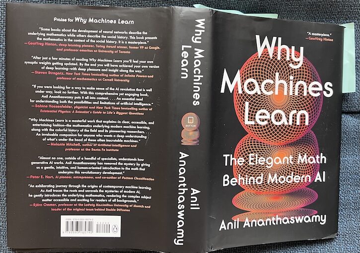
Why Machines Learn: The Elegant Math Behind Modern AI, Anil Ananthaswamy, 2024

November/December…, 2024

Context and Reflection

I am reading this book as part of a small book club: The 26-minute Book Club. This sort of book is really not my cup of tea — it is about the math with which various learning algorithms are implemented. I am, at my deepest, interested in the algorithms. Math is neither a strong point nor a deep interest — it seems more like magic to me: You generate a bunch of tautologies, define some terms and rules, and then elaborate it, and all of a sudden it enables you to do things.

I had imagined I would give this a one-meeting trial, and then bow out. However, I found the group (4 other people) quite pleasant, and composed of — barring the one person I know who invited me — interesting strangers that I would not otherwise get to know. And that, especially in retirement, is actually a pretty valuable thing. Everybody else I encounter is mostly a part of my social network.

Another advantage is that working through this book forces me to think about something that I would otherwise ignore: basic math including linear algebra, vectors, a little calculus, probability, gaussian distributions, Bayes’ Theorm. Perhaps it will prove tractable enough that I will feel emboldened to take on fluid dynamics, something that I suspect would help me better understand a whole range of natural patterns, from meteorological to geological…. Or perhaps I will figure out how to distill the ‘qualitative’ aspects that I am interested from the mangle of symbols. We shall see.

C1: Desperately Seeking Patterns

  • Konrad Lorenz and duckling imprinting. Ducklings can imprint on two moving red objects, and will follow any two moving objects of the same color; or two moving objects of different colors, mutatis mutandis. How is it that an organism with a small brain and only a few instants of exposure can learn something like this?
  • This leads into a brief introduction to Frank Rosenblatt’s invention of Perceptrons in the late 1950’s. Perceptrons are one of the first ‘brain-inspired’ algorithms that can learn patterns by inspecting labeled data.
  • Then there is a foray into notation: linear equations (relationships) with weights (aka coefficients) and symbols (variables). Also sigma notation.
  • McCulloch and Pitt, 1943, story of their meeting, and their model of a neuron — a neurode — that can implement basic logical operations.
  • The MCP Neurode. Basically, the neurode takes inputs, combines them according to a function, and outputs a 1 if they are over a threshold theta, and a 0 otherwise. If you allow inputs to be negative and lead to inhibition, as well as allow neuroses [sometimes spell-correct is pretty funny] to connect to one another, you can implement all of boolean logic. The problem, however, is that the thresholds theta must be hand-crafted.
  • Rosenblatt’s Perceptron made a splash because it could learn its weights and theta from the data. An early application was to train perceptrons to recognize hand drawn letters — and it could learn simply by ‘punishing’ it for mistakes.
  • Hebbian Learning: Neurons that fire together, wire together. Or, learning takes place by the formation of connections between firing neurons, and the loss or severing of connections between neurons that are not in sync.
  • The difference between the MCP Neurode and Perceptrons is that perceptrons input’s don’t have to be 1 or 0 — they can be continuous. And they are weighted, and they are compared to a bias.
  • The Perceptron does make one basic assumption: that there is a clear, unambiguous rule to learn — no noise in the data. If this is the case, it can be proven that a perceptron will always find a linear divide (i.e. when there is one to be found).

C2: We are All Just Numbers

  • Hamilton’s discovery of quaternions, and his inscription on Brougham bridge in Dublin. i2 = j2 = k2 = ijk = -1 Quaternions don’t concern us, but Hamilton developed concepts for manipulating them that are quite important: vectors and scalars.
  • Scalar/Vector math: computing length; sum; stretching a vector by scalar multiplication;
  • Dot product: a.b = a1b1 + a2b2 (the sum of the products of the vector’s components). The dot product (AKA the scalar product) is an operation that takes two vectors and returns a single number (a scalar). It’s a way to quantify how much two vectors “align” with each other — that is, the degree to which they point in the same direction.
    • E.g. Imagine pushing a model railroad car along some tracks. If you push in the exact direction that the tracks go, all the force you apply goes into moving the car; if you push at an angle to the tracks, only a portion of the force you apply goes into moving the car. This (the proportion of force moving the car along the tracks), is what the dot product gives you.
  • Something about dot products being similar to weighted sums, which can be used to represent perceptrons??? Didn’t understand this bit. [p. 36-42]
  • A perceptron is essentially an algorithm for finding a line/plane/hyperplane that accurately divides values into appropriately labeled regions.
  • Using matrices to represent vectors. Matrix math. Multiplying matrix A with the Transpose of Matrix B
  • So the point of all this is to take Rosenblatt’s Perceptron and transform it into formal notation that linearly transforms an input to an output.
  • Lower bounds tell us about whether something is impossible.” — Manuel Sabin
  • Minsky and Papert’s book, Perceptrons, poured cold water on the field by proving that Perceptrons could not cope with XOR. XOR could only be solved with multiple layers of Perceptrons, but nobody knew how to train anything but the top layer
  • I am not clear on why failure to cope with XOR was such cold water…
    Later: It is because XOR is a simple logical operation; the inability of Perceptrons handling it suggested that they would not work for even moderately complex problems. Some also generalized the failure to all neural networks, rather than just single layer ones.
  • Multiple layers requires back-propagation…

C3: The Bottom of the Bowl

  • McCarthy, Minsky, Shannon and Rochester organized the 1955 Dartmouth summer seminar on Artificial Intelligence. Widrow attended this seminar, but decide it would take at least 25 years to build a thinking machine,
  • Widrow worked on filtering noise out of signals: He worked on adaptive filtering, meaning a filter that could learn from its errors. Widrow worked on continuous signals; others applied his approach to filtering digital signals. Widrow and Hoff — Adaptive filtering — invented Least Mean Squares algorithm.
  • Least Mean Squares is a method for quantifying error. What Widrow wanted to do was to create an adaptive filter that would learn in response to errors — this required a method for adjusting parameters of the filter so as to minimize errors. This is referred to as The Method of Steepest Descent, discovered by the French mathematician, Cauchy.
  • Much of the rest of the chapter introduces math for ‘descending slopes.’ dx/dy moves us along a gradient… the minimum will have a slope of zero. When we have planes or hyperplanes we need to take multiple variables into account so we have partial derivatives.

“If there’s one thing to take away from this discussion, it’s this: For a multi-dimensional or high-dimensional function (meaning, a function of many variables), the gradient is given by a vector. The components of the vector are partial derivatives of that function with respect to each of the variables.

What we have just seen is extraordinarily powerful. If we know how to take the partial derivative of a function with respect to each of its variables, no matter how many variables or how complex the function, we can always express the gradient as a row vector or column vector.

Our analysis has also connected the dots between two important concepts: functions on the one hand and vectors on the other. Keep this in mind. These seemingly disparate fields of mathematics-vectors, matrices, linear algebra, calculus, probability and statistics, and optimization theory (we have yet to touch upon the latter two) – will all come together as we make sense of why machines learn.”

Reading Break…

  • So with an adaptive filter, you filter the input, and look at the error in the output, and feed that error back into the filter, which adjusts itself to minimize the error.
  • So first you need to be able to have an input where you already know what the true signal is, so that you can determine the error after the filter has transformed the input. How do you get that? ➔ Later: In the application we’re talking about, this is the training phase. Once the model is trained, you assume the characteristics of the noise will not change and the model will continue to work.
    One issue is whether the noise in the signal is always of the same sort — that is, if you train an adaptive filter on a bunch of inputs whose signals you know, will that give you a good chance of having a filter that can appropriately transform an unknown signal? The book uses the example of two modems communicating over a noisy line, and it makes sense (I think) that noise would have fairly uniform characteristics, at least for the session. But that seems unlikely to hold for everything.
    Can we assume that the noise, in a particular situation, is always the same ,or at least has the same statistical properties?
    Suppose the source or nature of the noise in the signal changes over time? Well, you could embed some kind of known signal into the input (I imagine, say, a musical chord), and let the filter learn to adjust the output so that the known chord comes through.
    But will a filter that preserves the chord also preserve the other information in the signal? I have no idea. I’d think it would depend a lot on (1) the nature of the signal, and (2) the nature of the noise.
  • I’m confused about the part about adding delays to signal… and I’m confused about how, in real life, you know what the desired signal is.
  • Later: Still not very clear on the noise issue, but I’m guessing it depends on what you’re applying it to. If the noise is varies in an unpredictable way for a particular application, then the filter/neuron simply won’t work and will produce gibberish.
  • Anyway, let’s assume we know the desired signal (and hence the noise/error) — how do we quantify the later? We don’t want to just add it up because it can have positive or negative values which would cancel one another out — instead, the errors are squared, and you take their mean to quantify the noise: the is called the Mean Square Error. It is also the case that squaring the errors exaggerates the effects of the larger errors, which seems like a desirable thing.
  • The math shows that the formula for the error associated with an adaptive filter is quadratic, meaning that it will be concave, and that thus the minimum error will be the minimum of the function. That can be found in multiple ways, either by finding the point at which the slope of the function is zero, or using gradient descent to find it.
  • A problem is that to do this, you need more and more samples of xn and yn and dn to calculate parameters, and you need to use calculus to calculate partial derivatives, and especially in high dimensional space this becomes burdensome (or impossible).
  • The solution was that Widrow and Hoff found a (IMO kludgy) way to just estimate the error without doing a lot of work.

weightNew = weightOld + 2 • <step-size> • <error-for-a-single-point>

  • This is called the Least Mean Squares (LSM) algorithm.
    Later: What they are doing is taking a single data point(a single input-out put pair) at random and using that to estimate the gradient and adjust the weight. Each update a new pair is randomly selected, and over time the algorithm noisily decreases the error. This is called Stochastic Gradient Descent. There is an alternative to this approach called mini-batch gradient descent that uses a randomly-selected set of points (e.g. 32 of them) for each update.

C4: In All Probability

  • The Monty Hall problem. There are three doors, one of which has a valuable prize behind it, and the others which have only goats. After you’ve picked door 1, Monty opens door 2, revealing a goat. You now have a change to change your pick — should you do that?
  • The answer. The answer is “yes.” For a long time this seemed counterintuitive to me (and Paul Erdos): revealing what is behind one of the doors should not change the probability of what is behind the other doors. What was tripping me up (ironically) is that I was ignoring the psychology. The key is that Monty is not opening a door at random: he knows what is behind each door, and in particular, he will not open a door that has the prize behind it (as that would destroy the game). So when Monty opens door 2, he is sometimes providing information about both door 2 and about door 3.
  • Let’s suppose I’ve picked the first door. There are three cases:
    (1) Pxx — if I have the correct door, Monty can open either of the others.
    (2) xPx — If a goat is behind 1, and P behind 2, Monty can only open 3
    (3) xxP — If a goat is behind 1, and P is behind 3, Monty can only open 2
    In 2 of these 3 cases, switching to the remaining unopened door gets me the prize. Monty has change the prior probabilities, and so we much re-evaluate.
  • This argument will hold for any number of doors, because Monty always knows where the car is, and since he will avoid opening that door, every door he opens changes the priors — i.e. gives additional information about the unopened doors.
  • Later: If we construct a different version of the problem, where, before Monty can pick a new door, an earthquake strikes and door 2 happens to collapse, revealing the goat, there is no reason to change (or not change) your pick. The revelation of the goat behind door 2 does not give us further information about what is behind any of the other doors, since the earthquake’s ‘revelation’ was truely a random event.
  • Bayes Theorem history. Interestingly, Thomas Bayes’ essay describing his approach was only presented to the Royal Society in 1763, two years after his death, by his friend Richard Price (who later scholars believe made substantive contributions, although Price attributed it all to Bayes).

P (X-is-true | given Evidence-for-X is positive)
IS EQUAL TO
P-X-in-the-world • How-strong-the-evidence-is (e.g. the accuracy of the test)
————————————- (DIVIDED BY) —————————————————-
(P-X-in-the-world • probability of a true positive)
• (1 – P-X-in-the-world) • (1 – probability of a true positive)

OR

The empirical probability in the world * the predictive accuracy given evidence
————————————————————————————————————————–
the likelihood of the world producing that evidence
(=sum of probabilities of all ways of producing that evidence)

Reading Break…

  • Machine Learning is inherently probabilistic because there are an infinite number of hyperplanes that can discriminate between a learned alternative, and it has settled on one of them for no particular reason. Other factors that make ML less than accurate are that the data itself may have errors, and that the amount of data drawn upon is limited. Later: And we must keep in mind that ML is only minimizing error — whether the result has enough signal to be useful is an empirical and domain-dependent issue.
  • Distinction between theoretical probability and empirical probability (e.g., theoretical probability of a fair coin coming up heads is 50%; empirical probability of a fair coin coming up heads depends on actually doing it, and it will approach but not reach the theoretical probability as one increases the number of empirical samples.
  • Aside: There is also the issue of the degree to which real-world events are actually expressions of mathematical distributions. It seems elegant to assume that, but is it really so?
  • The case of a coin flip is an example of a Bernoulli distribution. It has only two values, a and b, and can be characterized by a probability p that such that p is the probability of a, and (1p) is the probability of b.
  • Distributions with a mean and a variance (aka standard deviation). Now consider the case where you have N>2 outcomes, each with their own probability. This is distribution can be characterized by a mean and standard deviation — the mean (aka the expected value) is the sum of the values of each outcome multiplied by their probabilities, and the standard deviation is the square root of {the sum of the squares of the (deviations of each value from the mean)} — or the sum of the absolute value of each values difference from the mean. We can talk about the distribution as a whole in terms of its probability mass function.
  • So far we’ve been talking about variables with discrete values, but we can instead talk about variables with continuous values. Here we can’t talk about the probability of a particular value because there are an infinite number of values and the probability of any single perfectly precise value is zero. So, instead, what we do is talk about the probability of a value occurring within particular bounds: this is called the probability density function. [Aside: But wouldn’t it be possible to do some calculus like move where we look at what happens as a finite interval approaches zero?]
  • The important point is that whether we have a variable with discrete or continuous values, we can use well-known and analytically well understood functions to characterize the distribution.
  • Machine Learning. Let’s being with a set of labeled data points: y is a label that has two values, and x is an instance of the data. y is categorical; x is a vector with N components. This data set can be represented as a matrix: y1, x11, x12, x13 .. x1n and so on for y2, y3, etc. Each component of x is a feature that the algorithm will use to discriminate which y x belongs to.
  • Now, if you knew the underlying distribution P(y, x), you could determine the probability of y=A given x, and the probability of y≠A given x, and use the highest probability to assign the label. If this were the case, this is what would be termed a Bayes Optimal Classifier. [Aside: I’m a little unclear on this — it seems like it’s dependent on a particular situation, and so it seems odd to give it this sort of name.]
  • But usually you don’t know the underlying distribution, and so it must be estimated. Often it is easier to make assumptions about the underlying distribution (Bernoulli? Gaussian?), but it is important to keep in mind that these are idealizations chosen to make the math easier.
  • Aside: A Gaussian distribution is defined as being symmetric with respect to a single mode (which is also the mean and median), with asymptotic tails that never reach 0.
  • There are two approaches to estimating distributions:
    One is MLE or Maximum Likelihood Estimation, involves selecting a theta (that is a distribution with particular parameters indicated by theta) that maximizes the likelihood of observing (generating?) that labeled data you already have.
    In the text, MLE is exemplified by imagining a set of data about two populations’ heights, labeled short or tall, and that each population has a gaussian distribution, and thus that all the data will be best modeled by a combination of the two distributions. ???But is that still a gaussian distribution? And what is the rational for choosing a gaussian distribution rather than some other distribution???
    The other is called MAP, for Maximum A Posteriori estimation. As best I can tell, this involves estimating the distribution based on our experience of the world and representing it as a function. Then you set the derivative to zero, and solve that equation (after checking to be sure that you’ve got the maximum rather than the minimum). If this approach does not yield a ‘closed’ solution (most of the time), you can take the negative of the function and use gradient descent to find its minimum.
  • MLE vs MAP. So MLE tries to find the maximum using the data, and MAP tries to find the maximum of a distribution you’ve guessed at. MLE works best when there’s a lot of data; MAP works best when there isn’t much data you can make a reasonable guess about the underlying distribution).
  • The Federalist Papers example: which unattributed papers were written by Madison and which by Hamilton. A first approach was to analyze the length of sentences in papers know to be written by each author, and use the mean length and the standard deviation to discriminate: unfortunately the means and SDs for each author were almost identical. Later, someone suggested using the frequency of word use, and, in particular, function words tended to reliably discriminate between the known works of the two authors: this was then used to predict which of the unattributed essays were written by which author.
  • Aside: It is not clear to me whether the achievement of Mosteller and Wallace was due to the use of Bayesian reasoning, or to the realization the word choice was a very good discriminator between the authors. ➔ LATER: Consensus among scholar from many fields indicates, according to chatGPT, that their work did indeed validate the use of Bayesian inference, as well as creating a new approach to linguistics, and indicating the ways in which computers could be used.
  • The Penguin example.
  • A trick that statisticians use is to assume that the distributions for each feature under consideration are independent — seems like a bit of a leap, but it appears to work and it makes the math easier and requires less data.
  • Naive or Idiot Bayesian classifier.

… reading break…

C5: Birds of a Feather

  • The 1854 Snow Cholera Epidemic map
  • Voroni diagrams and nearest neighbors

… reading break…

Views: 0

Four Billion Years and Counting…

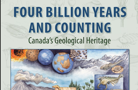
Four Billion Years and Counting: Canada’s Geological Heritage. Produced by the Canadian Federation of Earth Sciences, by seven editors and dozens of authors. 2014.

November-December, 2024.

I am reading this with CJS. It is a nice overview of regional geology, and it is nice that all the examples come from Canada, and at least some of the discussion is relevant to Minnesota Geology. The book is notable for its beautifully done pictures and diagrams.

The first part of the book, Foundations, is an introduction to general geological concepts. For CJS and I this will be largely review. Here I will preterit any summary, and simply list some of the points that stood out because they filled in a gap, or provided a different perspective.

FOUNDATIONS

Mostly background on geology for the general reader; but was good as a refresher, and also bringing in North American examples of various phenomena.

C1: On the Rocks

  • Polygonal jointing occurs when basalt flows stop moving before they cool.
  • Granitic magma forms at 600-900°, sometimes with water contributing to lowering the melting point, where silica minerals tend to melt, but more magic minerals remain solid. The melt tends to move upward, either because it is less dense than surrounding rock or because of tectonic pressures. As it forms a mass, chunks of surrounding “country rock” fall into it in a process called “stoping,” making the melt more silicacious and also persisting in solid chunks that will eventually become xenoliths.
  • Ripples (and their large scale cousins, dunes) are straight and symmetric if they are formed by currents moving back and forth, or curved if they are created by a unidirectional flow.
  • Mud cracks form as a result of repeated drying and wetting, as occurs in mudflats with seasonal rain, or intertidal areas.
  • A seam of coal that is a meter thick was originally 5-10 meters thick and took on the order of 2500 years to accumulate.
  • Paleosols, fossil soil surfaces/horizons, are generally rock-like with a characteristic disrupted knobby appearance.
  • Metamorphic rocks develop cleavage planes perpendicular to the direction force or pressure is being applied; metaphorphic rocks split along cleavage planes, not their original bedding surfaces.
  • Schist has a lot of mica; gneiss has little. Both are coarsely crystalline and so highly-altered that it is difficult to tell what the source rock was. The light and dark banding in gneiss is the result of recrystallization, and has nothing to do with the original bedding plane.

At lower metamorphic grades, platy crystals of chlorite and mica are common. As higher metamorphic grades are reached, minerals such as garnet, staurolite, and sillimanite may form. Such high-grade metamorphic rocks form at depths of 15 to 25 kilometres within the crust. If pressure (usually the result of deep burial) is a major factor during metamorphism, minerals such as kyanite and glaucophane may grow. The blue colour of glaucophane gives rise to the name blueschist, a rock formed under conditions of low temperature and high pressure.

Igneous rocks also show interesting metamorphic changes.When basalt is metamorphosed at low pressures and temperatures, some of its constituent minerals convert to the green minerals chlorite, actinolite, and epidote, producing a type of rock called greenstone or greenschist. At higher metamorphic grades, greenstone becomes amphibolite, a dark green to black rock made up of interlocking amphibole crystals.

C2: The Dance of the Continents

  • Reverse and thrust faults are different. They are created by the same array of forces, but reverse faults are steeper (closer to vertical) than thrust faults. …The text doesn’t say where the line is between them…
  • Fault breccia. Rock formed of a jumbled mix of sharp rock fragments embedded in lithified rock flour.
  • Nice review of minerals: pages 19-21.
  • The Greenville orogen underlies Quebec, the midwest US, and stretches into mexico.

All modern oceans contain areas where the lithosphere is thicker than regular oceanic litho-sphere. These areas include island arcs, oceanic plateaus perhaps bearing atolls, and isolated fragments of continental lithosphere such as present-day Madagascar. If subduction continues and these within-ocean features are swept toward the continent, they will ultimately collide with it. Because high-standing islands or plateaus are more buoyant than regular oceanic lithosphere, they will be scraped off the sub-ducting plate and will stick, or accrete, to the overriding plate rather than be subducted. Many mountain belts contain remnants of such former within-ocean features; such remnants are called terranes (a term not to be confused with terrain, which denotes topography). Terranes thus have a variety of origins: they may be continental fragments (microcontinents); former island arcs; or former pieces of thickened oceanic lithosphere such as Hawaii may become if it is accreted to a continent. Many terranes are a mixture of these elements. The convergence and collision of terranes with continental margins commonly leads to the rise of mountains.

Remnants of former deep oceanic lithosphere can be preserved within an ancient mountain system. Such remnants are known as ophiolite suites or ophiolites…

  • Rift Shoulder Highlands are mountains produced as a side effect of continental rifting — when the floor of the rift is bulging upwards.
  • Basins. Fore arc basins are in front of island arcs; back arc basins are behind them. Fore land basins can form on continents, due to the weight of accretionary material pushing down that part of the continental plate. …Is the Owens Valley in California such a basin?
  • The next supercontinent has already been named: Amasia.

…reading break…

C3: It’s About Time

This chapter was mostly review, but a few things stood out — either as needed reminders or new concepts/approaches.

  • Fission Track dating is possible with a mineral called Apatite. It contains small amounts of Uranium that disrupt the crystal structure, and whose decay produces scars. The scars ‘heal’ if it is heated much above 100° C, which can help determine, for example, when rock has been exhumed to surface levels and temperatures.
  • Thermoclock dating occurs in minerals which have small amounts of Uranium or Thorium. These isotopes decay, releasing Helium, and when the rocks has cooled below a certain temperature (dependent on the particular rock) the He can no longer escape, and thus the trapped He can be measured and the rock’s age determined.
  • Cosmogenic dating is possible when cosmic rays strike a rock on the surface and can alter the isotopes in it — for example, Beryllium. This technique can determine how long a particular rock surface (e.g. a glacial erratic) has been facing up.

C4: Fossils and the Brush of Life

Joseph Tyrell’s fishing trip to the Gunflint region — he sampled and later studied a black chert that had xxx Ga microfossils in it.

  • Types of fossilization: Permineralization is when pore spaces are permeated by mineral-bearing fluids which leave mineralization in the pore spaces; Replacement is when the material of the bone or shell is replaced by another mineral; Petrification is when both permineralization and replacement occur. In addition, molds or casts preserve the outlines of an organism, and trace fossils preserve a mold or cast of impressions made by organisms’ burrows, tracks, trails or footprints.

…reading break…

Part II: The Evolution of Canada

C5: From Stardust to Continents: Before 2.5 Ga

  • 4.567 Ga– – Solar System forms… quite precise for something that would seem to have fuzzy boundaries — did it really coalesce in a million years? …Or maybe that’s the oldest meteorites, and it was when the matter solidified enough to be datable…
  • 4.55 Ga — Age of most meteorites , which indicates that solar system did condense quite quickly, but not in a single million years!
  • 4.52 Ga — earth and a Mars-size body collided, giving the earth a ring that condensed into the moon; this also gave earth its 17° axial tilt
  • Initially the moon was less than a quarter of its current distance from the earth; and the earth was spinning faster, with 6 hour days. (And the sun was hotter as well.) The moon’s outer skin has largely been frozen since its early days.
    The Moon’s outer layers solidified from a global magma ocean roughly within the first 100–200 million years after its formation around 4.5 billion years ago, forming a stable, mostly anorthositic crust by about 4.4–4.3 billion years ago. The lunar mare basalts, which fill the large impact basins on the Moon’s surface, were emplaced significantly later, primarily between about 3.9 and 3.0 billion years ago, with some volcanic activity possibly continuing until as recently as 1.2 billion years ago.” [GPT]
  • 4.4 Ga — Earth had abundant water. Water carried into magma ocean below by sinking slabs led to a more silicic magma (with less magnesium and iron), and, being less dense, it tended to rise into the crust and form granitic plutons. Over time some would have risen to the surface, forming rafts of felsic rock that eventually got amalgamated into the first cratons.
  • 4.3-2.5 Ga — Craton formation
  • 3.5 Ga +/- 0.3 Ga — First evidence of life. (1) stromatolites; (2) mudstones with altered C12/C13 ratios indicating biological activity; (3) possible fossils of protists; (4) beginning of banded iron formations…
  • >2,6 Ga — komatiitie lavas
  • Basalt metamorphoses into greenstone (chlorite, actinolite) and that into hornblende.
  •  2-7 – 2.6 GaSuperior Craton forms — proto-continents welded together with oceanic lithosphere trapped between them.
    About 2,750 million years ago, the parts of the Craton underlain by granitic rocks (let’s informally call them protocontinents for simplic-ity) were separated by oceans, the width of which we can only guess. Around 2,720 million years ago, two protocontinents in the north (in terms of modern directions) collided, trapping a mixture of oceanic material between them. Around the same  time, other small protocontinents in the south amalgamated and were welded onto the northern block, sweeping up more tracts of oceanic lithosphere in the process. This amalgamation process, during which the oceanic material became compressed into the greenstone belts, continued until about 2,680 million years ago, by which time all the pieces of the Superior puzzle had come together.
  • 3.8 – 2.5 Ga — BIF (Banded Iron Formations). Differing theories for BIFs. One is that cyanobacteria produced O2 which led to oxidation of iron in ocean; (2) another is that early single-celled organisms used iron “to provide electrons for photosynthesis” producing oxidized iron.

…reading break…

C6: Laying the Foundations: 2.5 Ga to 750 Ma

  • Stanley Tyler discovers outcrop of Gunflint chert that is black and waxy-looking: This 1.9 Ga chert contains micro-fossils: thread-like filaments and hollow spheres on the order of a few microns across.
  • 2.5 – ~2 Ga — Breakup of Archean protocontinents (Slave and Superior cratons are remnants of these. This was accompanied by the formation of gigantic swarms of radiating dikes, possibly due to mantle plumes (e.g. Matechewan dike swarm in southern part of the Superior craton.
  • 2.5 – 2.4 Ga — The Great Oxidation event forms (among other things) beds of red sandstone. Note that the oxygen content of the atmosphere was still far less than it is today — a few percent (vs. 21%)
  • 2.45 – 2.2 Ga — Huronian tils provide evidence of first glaciation (in three waves)
  • 1.8 Ga – Nuna, first supercontinent forms.
  • 1.85-1.2 Ga — island arcs accrete on the southeast edge of Nuna. Also, in the interior, mountain ranges are weathering and sediment is being deposited in interior basins (e,g,, the Thelon and Athasbascan basins).
  • 1.09 – 1.0 Ga — Greenville orogeny (which involved collision of Amazonia (part of South America) with Laurentia) focused along what is now the southeastern flank of the Canadian shield. This was part of the assembly of Rodinia, and also possibly the genesis and termination of the mid-continent rift.
  • 1.0 – 0.750 Ga – Rodinia.
  • Passive margin sequences, from bottom to top (e.g. Huronian sequence in southern Quebec and Ontario exposed along trans-canada highway between Sudbury and Saute Ste. Marie):
    • rift-related coarse-grained sedimentary rocks possibly interlayered with or intruded by mafic volcanics. This stage of rift-filling often includes deposits of dense placer materials (e.g. uranite and pyrite) deposited where flowing streams slow down.
    • as the rift widens and sea floor spreading begins to form an ocean, there are finer grained and better sorted sandstones and mudstones.
    • as the ocean matures there are carbonate and chert layers (with stromatolites) from the shallow ocean floors

…reading break…

C7: Southern Sojourn: Canada 750 to 444 Ma

  • Discovery of Precambrian multi-cellular fossils in Newfoundland: aspidella and charniodiscus.
  • Cryogenian (850-630)=>Edicarian (630-542) =>Cambrian 542-488) =>Ordovician (488-444)

The Cryogenian

  • Rodinia => 780-750 Ma breakup…
  • Laurentia a separate continent by … experts disagree: 750-520 Ma. Anyway, over time, Laurentia, what was to become North America, was rotated 90° so that what is the east coast was oriented towards the paleosouth.
  • Windemere seaway rocks. A stack of sedimentary rocks that accumulate in a trough from California to Alaska — it is now found along the easter Cordillera. The stack includes deep water clastics, carbonates, and tillites with dripstones that were deposited in a rift basin (that perhaps evolved into a passive margin) — it can be seen in road cuts between Jasper, Alberta and Tete Jaune Cache BC, and also near Lake Louise.
  • Snowball earth? Tillites and dropstones occur at 740-670 Ma and 635-600 Ma. Paleomagentic data indicates that some of these sediments formed within 10° of latitude of the paleoequator. This is evidence for global glaciation, though many geologists are skeptical and favor a scenario where there re tracts of open ocean in which organisms would have been able to survive.
    • (If the earth was entirely glaciated, CO2 from volcanism would build up (because it would not be absorbed by the ocean or by surface weathering) and eventually a greenhouse effect would kick in).

The Edicarian

  • Metasoans appear ~ 580 Ma. Life prior to 580Ma (late Edicarian) was dominated by single-celled organisms; metazoans (multicellular animals with soft tissues in the form of disc-shaped, segmented or frond-like organisms) appeared as evinced by centimeter to meter scale fossils preserved in layers of sandstone or volcanic ash.

“While glaciers coated the world, the only organisms that fed on light beams were cyanobacteria. They thrived better than others in the oxygen-poor ocean, a relative nutrient desert. Only the freezing outflows of meltwater rivers carried enough oxygen into the seas for aerobic life to survive. As the snowball began to thaw, the melting ice wore away the continental surface, and drove millions of tons of phosphate into the ocean, creating a chance for an algal takeover. Suddenly, the advantage that cyanobacteria held – being able to absorb nutrients quickly because of their small size – was no longer relevant. Larger organisms were no longer outcompeted. and cyanobacteria were numerous enough to be preyed upon by larger microbes. Being big is an advantage for a predator, even one [that preys] on the microscopic cell, and it is at this time that multicellular algae became common .

– Thomas Halliday, 2022, (Otherlands, 273)

and also

“ In places the ground is coated with a firm, wrinkled layer, hardly distinguishable from the rest of the seabed except in texture, the folds of a rough rhinoceros-hide texture contrasting with the fresh-poured caster-sugar smoothness of ground quartz sand. The rough texture is the microbial mat, coating the interface between earth and water, an ecological structure that has already existed for billions of years. The two simplest domains of life, bacteria and archaea, have fed and reproduced at Ediacara for thousands of years, building layer upon layer as they stabilize the seabed, forming a coherent uppermost layer, like a skin on cold custard. Where the microbes are cyanobacteria, the mats often form distinct clumps called stromatolites that resemble slimy, slowly growing boulders, climbing their way to the light. Elsewhere, as in this delta, the mats are spread flat, a sheet of wrinkled life on the floor of the ocean. Only the top few layers are ever alive at any one time, but the combined generations of millions of microscopic cells nonetheless mean that the mats can reach thicknesses measured in inches. 

From these patches of microbial mat, strange, feathery shapes rise up to 30 centimetres into the water. Ridged, rugby-ball-shaped creatures, only a centimetre in diameter, drift between them. Above these hovers an eerie cone, a centimeter-scale flying saucer,   spinning as it drifts, before settling once again on the seabed. Close-up, it becomes apparent that this shadowy form is made of eight ridges, spiralling clockwise from the tip of the cone to its base, a coiling helter-skelter; floating hypnotically. Unable to move with great speed in the water, and hardly a natural swimmer, it nonetheless occasionally leaves behind its home on the microbial mat. It is found in the peace and quiet of the calm water below the storm base,and, when swimming, hangs in the water over stranger creatures still. Already, multicellular life is complex, and this is in fact one of the earliest creatures we can with certainty call an animal. Eoandromeda – so called because when flattened in fossilization, its eight arms resemble the spiral galaxy Andromeda – is a lantern in the Ediacaran murk, one of the few forms of life here that is remotely recognizable.”

– Thomas Halliday, 2022, (Otherlands, 275-6)

The Cambrian

  • The Cambrian Explosion, 542 Ma. Most sessile organisms became extinct by the end of the Edicarian, possibly due to the evolution of mobile organisms with a head end that allowed them to move forward. The first organisms with skeletons appeared around 550 Ma. The beginning of the Cambrian is marked by the appearance of trace fossils of worm burrows, and that was followed by the first “shelly” fossils. After that came brachiopods and archaeocyanthans, and then trilobites.
  • Oxygen explosion? One possible driver for the Cambrian explosion is that Oxygen increased to 3-10% (15-50% of present-day values). This is consistent with what analysis of contemporaneous sedimentary rocks show. Of course, it is also possible that the evolution of new morphological features — heads, eyes, mouths, teeth, segments, legs and antennae had something to do with it. …These features could have led to an evolutionary arms race as predators and prey engaged in a red queen’s race.
  • Protichnites. In 1983 trace fossils of an arthropod walking on land were discovered in a quarry nears Kingston, Ontario, in 500 Ma sandstone formed from aeolian dunes. This is tens of millions of years before any other animals are known to have walked on land, so perhaps this was just a temporary outing!
  • paleo-South: Rifting / opening of Iapetus (circa 600 Ma), and microcontinent suturing. Around 600 Ma crustal rifting began to separate Laurentia from Amazonia, forming rifts that can still be seen in the valleys of the St Lawrence and Ottowa rivers. As time went on (moving into the Ordovician) microcontinents — Gander, Avalonia and Magma accreted to the paleo-southern shore of Laurentia (now east coast of North America).
  • paleo-East (north): Spreading opens Ural Ocean (circa 600 Ma). From 600-480 Ma this was a passive margin that accumulated carbonates which are still preserved as flat strata overlying artic islands. This margin area may have been quite shallow, as there are extensive deposits of evaporites. Between 480-450 Ma a subduction zone and magmatic arc developed in the Ural ocean, leading to the creation and eventual accretion of amicrocontinent called Pearya to the paleo-east side of Laurentia later on…
  • paleowestern (southern) margin. The core of Laurentia has been stable since the Grenville Orogeny — it is called the North American Continental Platform.

Ordovician

  • Brachiopods proliferated and nauteloids rose to prominence. Trilobites continued to thrive, as did echinoderms, especially crinoids.

…reading break…

Box 6: The Burgess Shale

  • The Burgess Shale (named for a nearby mountain and pass) is near the town of Field in the Southern Canadian Rockies and is renowned for its preservation of a menagerie of 505 Ma fossils of soft-bodies animals. it is now a UNESCO World Heritage Site.
  • Fossils in an area called “the trilobite beds” were discovered near Mt Stephen during the construction of the railroad, and Canadian paleontologists identified and characterized a number of the fossils. But it was not until Charles Walcott, an American paleontologist and secretary of the Smithsonian Institution, did further exploration in the area, that the Burgess Shale itself was discovered. Between 1910 and 1924 Walcott and his family collected around 65,000 specimens (!!!!!) from the shale.
  • The Royal Ontario Museum’s Burgess Shale collection contains more than 150,000 fossils.
  • The Burgess Shale has yielded fossils, often exquisitely preserved, even to the extent of preserving gut contents, of more than 200 organisms, most of which lack shells. The fossils yield great insight about the morphology of Cambrian organisms: some appear familiar to us, others demonstrate mixtures of body parts that strike us as odd and outlandish. For example, Opabina has five eyes, an extended proboscis, a segmented body, and no legs.
  • The Shale also offers interesting case study in how fossils have been reinterpreted over time. For example, Anomalocarius Canadences (“Canada’s odd shrimp”) turns out to have been the claw of a larger organism (but which still retains the original name). Similarly, many of the fossils which were once considered to be representatives of extinct phyla are now thought to be early branches of existing phyla.
  • Stephen Jay Gould’s book, Wonderful Life, is about the Burgess Shale.
  • The Shale appears to be the result of periodic mud slides in the ocean that buried and instantly killed (because no evidence of escape attempts) the organisms, and preserved them in an anoxic environment.

Box 7: The Green Revolution

  • Chloroplasts were originally prokaryotic cyanobacteria that were engulfed and incorporated into early plant cells. Note that some cyanobacteria still survive independently.
  • Several lineages of algae developed multi-cellular forms independently. They also trapped or incorporated different pigments — red and brown chlorophylls are predominantly found in sea weeds; green is as well, though it is also what gave rise to land plants.
  • Freshwater forms of green algae invaded land on many occasions, but only one — embryophytes, was really successful on land. The key was adaptations that allowed plants to live in open air, and deal with dessication. In water, plants can easily obtain food and water by absorption directly into their cells, expelling wastes which diffuse away, and enjoy protection from UV light and neutral buoyancy for support. None of these advantages obtain on land.
  • Embryophytes include plants from the simple lungwort to the deciduous trees.
  • The first land plants were likely bryophytes such as mosses — they don’t have a vascular system or roots, and thus require moist environments, but they do use spores as a reproductive mechanism. These appeared in the Ordovician, about 470 Ma.
  • In the Silurian, at about 425 Ma, tracheophytes — plants with a superior vascular system — appeared. This includes most of the plants we’re familiar with, from ferns to trees. The vascular system both provided means for transporting water and nutrients within the plant, and also mechanical support so that they could compete for light and withstand environmental forces.
  • Leaves, wood and seeds appeared in the Devonian (xxx Ma)
  • Leaves may have been a response to declining CO2 levels during the Devonian and enabled the plant to take in sufficient CO2.
  • Wood enabled plants to grow taller, and by the late Devonian forest canopies had replaced knee-high thickets.
  • Seeds, by providing a store of water and nutrients, enabled plants to reproduce in drier environments (e.g. where there were seasonal rains and dry periods.)
  • Around the Carboniferous-Permian boundary (300 Ma), the global environment became much drier, and conifers and cycads became the predominant phyla.
  • Later (140 Ma) flowering plants came on the scene, and are now one of the most successful types.
  • Grass, a type of flowering plant but different in that it is predominantly wind-pollinated, appeared only 25 Ma during the Oligocene. It was adapted to the dry environments of continental interiors, possibly because of a different photosynthesis pathway. [check]

C8: Crossing the Equator

  • This chapter:
    Silurian(444-416)=>Devonian(416-359)=>Carboniferous(359-299)=>Permian(299-251)
    • Laurentia fused with Gandara and Baltica to form Euramerica, which then began to rotate [???] counterclockwise until its present eastern margin faced paleosoutheast. The most important point is that what was to become north america was actively rotating and drifting north. By 315 Ma the paleoequaor was crossing through the SW US and eastern Canada.
  • 310 Ma: Euroamerica and Protogondwana had come together, forming Pangea, though Siberia was a bit late to the game.
  • Collisions
    • 1. 480 Ma: Dashwood microcontinent accretes to south short of Laurentia in the Taconic orogeny, the first in the series of orogenies that produced the Appalacheans.
    • 2. 440-422 Ma: Gandaria collides with southern Laurentia in the Salinic orogeny. Then in 420-390 Ma Avalonia collides with the Gandarian margin of Laurentia in the Arcadian orogeny.
    • 3. 390 Ma. Meguma is pulled sideways against Avalonian margin in the neoarcadian orogency
  • xxxx

…reading break…

Views: 11

Through the Language Glass

by Guy Deutscher

October 2024

This is an excellent book; interesting well-documented science, and some beautiful and erudite writing as well. The basic argument — that grammar determines what must be specified, rather than what can be specified, and in that manner instills certain habits of mind that effect how people see the world — seems correct, if not quite living up to the subtitle of the book: Why the World Looks Different in Other Languages.

Perhaps the most interesting and fun part of the book was to be introduced to languages that work very differently from English: The Mates language (in Peru) that requires speakers to specify whether the fact they report is based on personal observation, indirect evidence, or hearsay; and the Australian language that has no egocentric prepositions, but requires all positional information to be reported in terms of the cardinal directions, thus requiring their speakers to always be oriented.

This book was a pleasure to read. I plan to seek out other work by this writer. 

Contents

Front Matter

On whether languages reflect the characteristics of their speakers, he writes:

Many a dinner table conversation is embellished by such vignettes, for few subjects lend themselves more readily to disquisition than the character of different languages and their speakers. And yet should these lofty observations be carried away from the conviviality of the dining room to the chill of the study, they would quickly collapse like a soufflé of airy anecdote-at best amusing and meaningless, at worst bigoted and absurd.

— p. 2

The basic argument of the book is this:

The effects that have emerged from recent research, however, are far more down to earth. They are to do with the habits of mind that language can instill on the ground level of thought: on memory, attention, perception, and associations. And while these effects may be less wild than those flaunted in the past, we shall see that some of them are no less striking for all that.

I think it is correct, but that the subtitle of the book – Why the World Looks Different in Other Languages – is a bit of an exaggeration.

C1-5: <Reprise of history and status of color terms>

C1: Naming the Rainbow

This chapter reprises now-unknown work by William Gladstone (now remembered as an English prime minister) on Homer and his writings, and focuses in on particular on one chapter in Gladstone’s monumental 3,000 page work: a chapter on Homer’s use of color terms.

Gladstone’s scrutiny of the Iliad and the Odyssey revealed that there is something awry about Homer’s descriptions of color, and the conclusions Gladstone draws from his discovery are so radical and so bewildering that his contemporaries are entirely unable to digest them and largely dismiss them out of hand. But before long, Gladstone’s conundrum will launch a thousand ships of learning, have a profound effect on the development of at least three academic disciplines, and trigger a war over the control of language between nature and culture that after 150 years shows no sign of abating.

Gladstone notes that Homer uses color terms in odd ways — the famous “wine dark sea” (really “wine-looking” sea) being just one example.

Mostly Homer, as well as other Greek authors of the period, use color very little in their descriptions: mostly they use black or white; terms for colors are used infrequently and inconsistently. For example, the only other use of “wine-looking” is to describe the color of oxen.

Gladstone’s fourth point is the vast predominance of the “most crude and elemental forms of color”-black and white-over every other. He counts that Homer uses the adjective melas (black) about 170 times in the poems, and this does not even include instances of the corresponding verb “to grow black,” as when the sea is described as “black-ening beneath the ripple of the West Wind that is newly risen.” Words meaning “white” appear around 100 times. In contrast to this abun-dance, the word eruthros (red) appears thirteen times, xanthos (yellow) is hardly found ten times, ioeis (violet) six times, and other colors even less often.

C6: Crying Whorf

This chapter describes the origin, rise and fall of linguistic relativity. Sapir is depicted as respectable but making over-stated claims; Whorf comes across as a charlatan, for example, making claims to have deeply studied Hopi, when he only had access to a single informant in New York – and making broad claims that are entirely wrong (e.g. that the Hopi language does not have a future tense). 

Deutscher traces the origin of linguistic relativity to Wilhelm von Humboldt in 1799,  whose “linguistic road to Damascus led through the Pyrennes.” Deutscher encountered the Basque language, and found that it was radically different from the languages linguists tended to study. He then sought out other ‘more exotic’ languages, which he found by going to the Vatican library and studying the notes of Jesuit missionaries to South and Central America: “…Humboldt was barely scratching the surface. But the dim ray of light that shown from his materials felt dazzling nonetheless because of the utter darkness in which he and his contemporaries had languished.” p. 135 Although Humboldt’s ideas led to linguistic relativity, it should be noted that he had a much more nuanced and correct view: In principle, any language may express any idea; the real differences among languages are not what they are able to express but in “what it encourages and stimulates its speakers to do from its own inner force.” But this view was not carried forward, and instead: “The Humboldtian ideas now underwent a process of rapid fermentation, and as the spirit of the new theory grew more powerful, the rhetoric became less sober. ”

All that said, Deutscher argues it is a mistake to dismiss the idea that language has no influence over thought. But rather than taking the strong case the language constrains thought, he instead argues the habits of language may lead to habits of mind. In the case of the influence of language, and refers to the idea that Boas introduces and that Jakobson crystalized into a maxim: “Languages differ in what they must convey, and not in what they may convey.”

Phrases I like

“…has still the power to disturb our hearts.” [Sapir, referring to Homer, Ovid, etc.] p. 129

“[His] linguistic road to Damascus led through the Pyrennes.” p. 134

“…Humboldt was barely scratching the surface. But the dim ray of light that shown from his materials felt dazzling nonetheless because of the utter darkness in which he and his contemporaries had languished.” p. 135

Views: 3

w/CJS: Best Science & Nature Writing, 2022

Reading The Best American Science and Nature Writing , 2022 (ed. Ayaba Elizabeth Johnson) with CJS.

So far, as of May 2024, this is a very enjoyable read. I particularly appreciate the efforts of the editor to create a nice progression of topics, giving what is essentially an eclectic sampling of articles a higher level narrative.

September 2024: Nearing the end; still an enjoyable read.

Favorites

After finishing the book, here are my favorites

Top Five Six

  • C2 – What Slime Knows. Really gave me a new view of slime molds. I hadn’t realized the degree of intelligence a seemingly simple colonial organism can possess. Offers a counter-narrative to the usual ideas about what is necessary for intelligence.
  • !! C7- Rising Groundwater. This is the biggest eye-opener in the book, at least for me. While sea level rise will have very obvious impacts on costal regions, this makes the point that sea water will also cause a rise in ground water and, with or without infiltrating it, will cause a lot of problems for a lot more people than are effected directly by sea level rise. Think corroding water and gas pipes, malfunctioning sewage systems, and failing electical systems. This is one I’ll tell other people about.
  • C15: Poisoned—Part I: The Factory. Not a pleasant story. Talks about working conditions in a battery recycling factory, the horrible degree of exposure to lead, and the toll it takes on the workers. Shocking for two reasons: one is that the company behind this is based in Minnesota, and is in theory doing good things (recycling lead from batteries); second, that the industry and factories are regulated, but that in spite of that conditions are horrible.
  • !! C25 – Why Combining Farms & Solar Panels Could Transform How We Produce Both Food and Energy. A hopeful and plausible tale about how we can do better quite easily. A win-win. Perspective shifting and positive. I’ll mention this to others.
  • : – ) C28 – Beavers Are Firefighters Who Work for Free (Sierra) A perspective shifting article on role beavers can play in making land more resistant to wildfires, and also points out that the autonomy of tribes can allow them to take the forefront in experimenting with more sustainable approaches to environmental problems.
  • : – ) C32 – A River Reawakened (Orion). Not a perspective shifter, but just a very pleasant positive piece on what happens when a river is undammed, the problems that need to be addressed, and the rapidity of recovery. This was going to be an honorable mention, but I liked it too much!

Honorable Mentions

Continue reading w/CJS: Best Science & Nature Writing, 2022

Views: 14

w/RB: The Master Builder: How the New Science of the Cell is Rewriting the Story of Life, Alfonso Martinez Arias

* The Master Builder: How the New Science of the Cell is Rewriting the Story of Life, Alfonso Martinez Arias, 2023

March 2023…

I am reading this book with RB, a chapter or two at a time. My first impression is that it is going to be a great read. It has interesting and new-to-me science straight from a scientist who has spent his career studying this area, and it is well written too.

The premise of the book is that DNA gets too much credit for its role in shaping organisms, and that it is also important to pay attention to the ways in which cells carry out the ‘instructions’ of DNA. Unlike DNA, cells can respond to their environment, sense ambient conditions at the cellular level, and respond to distance and orientation. Quite a number of things that we would presume would be determined by genetics — everything from finger prints and retinal patterns to birth defects, propensity to diseases, and the location of organs in the human body — are determined by cells rather than DNA.

Continue reading w/RB: The Master Builder: How the New Science of the Cell is Rewriting the Story of Life, Alfonso Martinez Arias

Views: 18

LS: A Wilder Time,* William E. Glassley

*A Wilder Time: Notes from a Geologist at the Edge of the Greenland Ice. William E. Grassley, 2018.

A lyrical book that provides an account of a geologic expedition to gather evidence for a 1.8 Ga collision between continents that resulted in a series of shear zones in western Greenland. Also important for providing evidence that plate tectonics has been going on for a long time, something that has been contested. Content is quite interesting, but I also appreciate it for its lyrical writing about landscape and geology, which is this focus of my “LS” project.

Continue reading LS: A Wilder Time,* William E. Glassley

Views: 12

EP#14: 2023 Best Science & Nature Writing–Overview

* The Best American Science and Nature Writing of 2023 (ed. Carl Zimmer)

February – March 2024

CT and I selected this book to continue our essay project. However, after reading the first three pieces, we have reconsidered. Although the articles are interesting, they are not what either of would call essays. It’s really journalism, with the focus on ideas. The prose is generally clear and workman like, but as yet we have not encountered any writing that makes us pause to savor the phrase. We intend to look through the book, and — by paying attention to where the piece was originally published – see if we can come up with more essay-like pieces. However, we both suspect, that the book will not past muster vis a vis our project, and that we will move on to something else following our next meeting.

Continue reading EP#14: 2023 Best Science & Nature Writing–Overview

Views: 40

LS: Land Above the Trees: A Guide to American Alpine Tundra, Ann Zwinger & Beatrice E. Willard

February 2024…

This book was recommended in Kim Stanley Robinson’s The High Sierra: A Love Story, as a good guide to the ecology and botany of the Sierra Nevada (and the upper portions of other North American ranges). And, indeed, it is beautifully written with a narrative style in which the reader moves through landscapes with the authors, looking at this and that, in contrast to what I had expected would be more of a catalog or encyclopedic approach. The book is divided into two principle parts: part 1 examines elements of ‘above the trees’ ecosystems, like fellfields or krumholtz; part 2 looks at particular North American tundra ecosystems, with one chapter being on the Sierra Nevada.

Continue reading LS: Land Above the Trees: A Guide to American Alpine Tundra, Ann Zwinger & Beatrice E. Willard

Views: 13

w/CS: Gulp: Adventures on the Alimentary Canal, Mary Roach

January-February 2024

Gulp: Adventures on the Alimentary Canal, Mary Roach, 2022. I am reading the with CS. Mary Roach is a popular science writer who has developed a ‘brand’ of doing popular science books with toungue-in-cheek titles like Gulp, Stiff, Bonk, and so forth.

My impression after the first two chapters is that it will be a fun, fairly light read. She is very good at tossing in the amusing descriptive phrase.

Continue reading w/CS: Gulp: Adventures on the Alimentary Canal, Mary Roach

Views: 21

EP #`13: Awakenings, Oliver Sacks

January 2024

Entry 13 in the Essays Project with CT; this is the seventh book we’ve read by Oliver Sacks. This is the book that, with the help of a documentary and then movie, transformed him into something of a celebrity. It is an account of the experience of ‘awakening’ patients with Parkinson’s induced by Encephalitis Lethargia by administering L-Dopa, their experiences of returning to a sort of normal life, and then their declines due to the follow-on negative effects of L-Dopa.

Continue reading EP #`13: Awakenings, Oliver Sacks

Views: 33

LS*–The High Sierra: A Love Story, Kim Stanley Robinson

November 2023

The High Sierra: A Love Story, by Kim Stanely Robinson. 2022.

* I was reading this for other reasons, but nevertheless it fits well into my project to read essays that focus on landscape and natural history.

TL;DR: I love this book. But it is not for everyone. On the other hand, it is organized in such a way that readers interested in particular topics — geology, history, etc. – could skip through the book attending to one or a few themes that interest them. It has great pictures, too.

#

I’m a big fan of KSR, and think it likely that I’ve read everything he’s written, although it is possible that that omits a few early science fiction novels that were retroactively published after he became better known. I like the complex characters he develops, the intensely developed worlds he portrays, and especially his attention to geology, climate, economics, politics, and the role of large institutions – themes that are uncommon in much science fiction. Also unusual is that he sometimes ventures beyond the borders of SF, as with his novel Years of Rice and Salt, and especially with this book, which is multi-threaded work the interweaves memoir, geology, natural history and history.

Continue reading LS*–The High Sierra: A Love Story, Kim Stanley Robinson

Views: 23

w/CS: Elixir: A History of Water and Humankind*, Brian Fagan

November 2023…

*Elixir: A History of Water and Humankind, Brian Fagan. Reading with CJS.

Comment after finishing seven chapters:
There is interesting material here, and I am happy to be reading it. However, the writing is not grea: it is difficult to follow if you are really trying to get a deep sense of what is going on.

  • The same date is sometimes referred to as 4,000 BCE, 6,000 years ago, or a millennia after another event. I can do the math, but pausing to do so drops me out of the flow of the text.
  • The maps helpfully included in the chapters lack many of the places referred to in the text: Where are the Taurus mountains? Are they the same as the mountains near Cudi Dag (not shown on the map either). Clearly, neither writer nor editors ever tried referring to the associated map…
  • Places are also referred to with different names: The Lands of Enlil; Southern Mesopotamia; the lands to the south of modern-day Bagdad; the Fertile Crescent refer, I think, to the same area. But it is difficult to be sure.
  • Often it is unclear what the relationship between sequential examples are — are they supposed to reinforce one another, or complement one another, or are they being presented for some other reason? Sign-posting would be really helpful.

Preface

The three themes of this book are (1) gravity and its fundamental impact on the flow of water; (2) the relationship between ritual and water management; and (3) sustainability. One point the book will take up is the way in which the invention of the mechanical pump transformed the mining and movement of water.

The book takes an anthropological perspective, closely examining the relationships between water technologies and human usage and management practices, and looking at the role rituals play. It looks at both historical examples — even reaching into the deep past where the primary source of information is archeological work — and present day examples. And of course the book addresses the ongoing crisis in water sourcing and distribution, and the question of sustainability.

Continue reading w/CS: Elixir: A History of Water and Humankind*, Brian Fagan

Views: 22

EP#12: The Mind’s Eye, Oliver Sacks

Entry 12 in the Essays Project with CT; and this is the sixth book we’ve read by Oliver Sacks. Here we take up the neurological case account essays for which he is best known, after reading his two autobiographies, and other writings ranging from general essays to an account of his travels in Oaxaca. This book, published in 2010, explores cases in which people have lost visual abilities that we all take for granted – not so much blindness (although maybe there will be some essays on that), but rather the consequences of some of the many ways in which the complex and intertwined elements of the visual processing system may be disrupted.

Continue reading EP#12: The Mind’s Eye, Oliver Sacks

Views: 13

w/CS: Islands of Abandonment: Nature Rebounding in the Post-human Landscape, by Cal Flyn

September 2023

Islands of Abandonment: Nature Rebounding in the Post-human Landscape, by Cal Flynn, 2021.* This book looks at how nature — fungi, plants, animals – are re-colonize landscapes that have been destroyed and abandoned by humans. Examples include massive slag piles, nuclear test grounds, etc. It examines both how primary succession occurs in unpromising circumstances, and how the absence of human presence facilitates re-wilding. In the introduction, the author notes that we are now in the midst of a vast self-directed experiment in re-wilding, driven in part by the concentration of people in cities (and a soon-to-be-decreasing population), and in part by the depletion of non-sustainable natural resources that leave ‘waste lands’ behind.

Post-reading comment: There are three or four chapters in the book that are great, and really align with the aims laid out above. Unfortunately, more of the chapters, particularly as one progresses in the book, are more in the line of what I would call disaster tourism: lyrical descriptions of degraded environments and terrible situations, with little or no mention of how the ecosystem has adapted or not.

* Reading with CJS, fall of 2023

Continue reading w/CS: Islands of Abandonment: Nature Rebounding in the Post-human Landscape, by Cal Flyn

Views: 15

w/RB: An Immense World: : How Animal Senses Reveal the World Around Us, Ed Yong

An Immense World: How Animal Senses Reveal the World Around Us, Ed Yong, 2022.

Overall, a good book. Yong writes well, and sometimes has very nice turns of phrase, though I’d say his gift is more for clarity and content than lyricism. The downsides of the book — small ones but nevertheless there — is that he often doesn’t go as deeply into the mechanisms and neurophysiology of sensing as I would like. It is also the case that one gets a bit of whiplash from looking first at this organism, and then at that, and then at that — but I don’t see how that could have been avoided in this sort of book.

To summarize briefly and incompletely, here are some of the points I found most interesting:

  • What we think of as a single sense (e.g., vision) can be quite complex. All of the following can be separate: distinguishing light from dark areas; color vision (and bi- tri- and tetra-achromatism); ability to see polarized and/or UC and/or infrared light; and more.
  • Also, the same sense can be configured and deployed in different ways: the shape of an organism’s visual field is tightly bound with its role in the food web; an organism may have one, two or multiple eyes, and may be able to move them independently; and so on.
  • Some senses seem easy to evolve, in that they have been independently evolved at many different points in time. And then lost, and then re-evolved.

April 2023 – February 2024

Introduction

The book begins with a fanciful description of a room with different creatures in it, including a human, a robin, an elephant, a spider, and so on. It uses this to make the point that the different creatures, although all in the same room, have radically different impressions of the room and its occupants. What is evident to one is invisible to another. An organism’s very particular view of its environment – is referred to as its umveldt, coined by Jacob Uexkull in 1909.

Continue reading w/RB: An Immense World: : How Animal Senses Reveal the World Around Us, Ed Yong

Views: 37

w/CS: The Ends of the World, Peter Brannon

The Ends of the World: Volcanic Apocalypses, Lethal Oceans, and our Quest to Understand Earth’s Past Mass Extinctions. Peter Brannon. 2017

April – June 2023

Summary of Periods and Mass Extinctions

  • Edicarian: 635-538. First appearance of wide-spread multi-cellular organisms in ocean: Soft-bodied microbial organisms forming mats and other structures, and free-floating filter feeders.
  • End-Edicarian extinction: ~448. 86% species went extinct.* Possibly due to advent of burrowing organisms that disrupted largely sessile ecosystem. Not an official mass extinction because of a very incomplete fossil record.
  • Cambrian: 538-485. Warm shallow seas flank margins of several continental remnants of the breakup of the supercontinent Pannotia. In ocean there is the advent of hard-bodied complex organisms, and subsequent explosion of diversity into all phyla known today. The land bare except for microbial crust; arthropods and mollusks begin to adapt to life on land towards the end of this period.
  • Ordovician: 485 – 433. High CO2 levels and continents inundated with vast shallow seas jammed with life: brachiopods; trilobites; cephalopods; eurypterids; grapholites; and jawless fish. Many isolated continents and islands, with continents at south pole and a global sea occupying most of the northern hemisphere. First spores of land plants (fungi and simple plants) at 467Ma, with their spread possibly releasing phosphorous into the ocean stimulating algal blooms and CO2 sequestration.
  • End-Ordovician extinction:~345 Ma. 75% species went extinct.* Major ice age, likely precipitated by biogenic CO2 depletion, followed by a whip-lash of warming.
  • Silurian: 443-419. Gondwanaland and island chains provide diversity of environments; in the ocean early fish diversify into jawed and bony fish. Terrestrial life expands in the Silurian-Devonian Terrestrial Revolution: vascular plants emerge from more primitive land plants, and three groups of arthropods (myriapods, arachnids and hexapods) became fully terrestrialized.
  • Devonian: 419-359. Gondwana supercontinent in the south, Siberia to the north, and Laurussia to the east. Free-sporing vascular plants form extensive forests (Archaeopteris); by the middle of the Devonian several groups have evolved leaves and true roots; by the end the first seed-bearing plants appear.
  • Late-Devonian extinction event: ~250 Ma. 96% species went extinct.* Two major extinction pulses, and many smaller pulses. One theory is that it is due to the release of nutrients by the punctuated spread of land plants as they developed vascular systems with leaves and roots, and seeds.
  • Carboniferous: 359-299. Age of amphibians — also first appearance of amniotes from which both reptiles and mammals came. Vast rainforests covered the land, and insects diversified. The latter part of the Carboniferous experienced glaciations, low sea level, and mountain building as the continents collided to form Pangaea. A minor marine and terrestrial extinction event, the Carboniferous rainforest collapse, occurred at the end of the period, caused by climate change
  • Permian: 299-251. On land: The Carboniferous rainforest collapse left behind vast regions of desert in the continental interior. Amniotes, which could better cope with the conditions, diversified into the synapsids (the ancestors of mammals which came to dominate the Permian) and the sauropsids (reptiles). . In the ocean fish diversify with placoderms dominating almost every known aquatic environment, alongside coeleocanths, with sharks and bony fishes on the sidelines.
  • End-Permian extinction: 251.9 Ma. 80% of species went extinct.* The Siberian Traps were created at 252 Ma and also interacted with the Tunguska sedimentary basin filled with carbonates, shale, coal and salt in layers up to 12 Km thick; it is the worlds largest coal basin. When the magma intersected the basin, it caught fire, detonated in multiple places, and released vast about of CO2 and methane, on top of the CO2 produced by the eruption contributing to global warming and ocean acidification and anoxia. Other chemicals produced by the incineration of the Tunguska basin contents may have destroyed the ozone layer.
  • Triassic: 252-201. Brannen argues for a long 5 – 10 million year recovery, but that is disputed. The ancestors of crodcodiles dominated the Triassic; ancestors of dinosaurs and first true mammals appear, but were not dominant. The global climate during the Triassic was mostly hot and dry. Pangea had deserts spanning much of its interior until ita began to gradually rift into Laurasia and Gondwana to the south. In line with this the climate shifted from hot and dry to more humid, with a massive rainfall event called the Carnian Pluvial Event that lasted a million years.
  • End Triassic Extinction: 200 Ma. 80% of species went extinct.* Volcanism from the rifting of Pangea produced flood basalt that covered more than 4 million square miles. The CO2 concentration doubled or tripled, raising the already warm temperatures by at least 3 ° C. The final extinction pulse was fast: on the order of 20,000 years.
  • Jurassic: 201.4 – 145. Gondwana begins to rift. Climate warm and humid.
  • Cretaceous: 145 – 66. Gondwana completes rifting and by the end of the period today’s continents are recognizable, but with shallow inland seas in North America and Africa and between Greenland and Norway.
  • End Cretaceous Extinction: xxx. 76% of species went extinct.* Most likely some combination of the eruption of the Siberian Traps and the Chixtulub impact lead to global warming and an extended period of darkness. Almost all large animals eliminated, including all dinosaurs excerpt ancestors of birds.
  • Percent of species that went extinct, for any one event, vary considerably among sources. These numbers are better read as an indicator of relative severity.
Continue reading w/CS: The Ends of the World, Peter Brannon

Views: 18

w/CS: The Tangled Tree: A Radical New History of Life, David Quammen

January – April 2023

The Tangled Tree: A Radical New History of Life, David Quammen, 2018. These are my chapter by chapter notes. Besides having very good reviews and being by a well-regarded author, this book got a (rare) very high rating from Reid Priedhorsky…

Read this with CS.

Continue reading w/CS: The Tangled Tree: A Radical New History of Life, David Quammen

Views: 10